Functions

This module contains the algorithms for the linear equations lab.

The materials follow Miranda and Fackler (2004, [MF04]) (Chapter 2). The python code heavily draws on Romero-Aguilar (2020, [RA20]) and Foster (2019, [Fos19]).

labs.linear_equations.linear_algorithms.backward_substitution(a, b)[source]

Perform backward substitution to solve a system of linear equations.

Solves a linear equation of type $Ax = b$ when for an upper triangular matrix $A$ of dimension $n \times n$ and vector $b$ of length $n$ .

Parameters

a (numpy.ndarray) – Lower triangular matrix of dimension $n \times n$ .
b (numpy.ndarray) – Vector of length $n$ .

Returns

x – Solution of the linear equations. Vector of length $n$ .

Return type

numpy.ndarray

labs.linear_equations.linear_algorithms.forward_substitution(a, b)[source]

Perform forward substitution to solve a system of linear equations.

Solves a linear equation of type $Ax = b$ when for a lower triangular matrix $A$ of dimension $n \times n$ and vector $b$ of length $n$ . The forward subsititution algorithm can be represented as: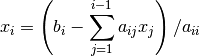

$x_i = \left ( b_i - \sum_{j=1}^{i-1} a_{ij}x_j \right )/a_{ii}$

Parameters

a (numpy.ndarray) – Lower triangular matrix of dimension $n \times n$ .
b (numpy.ndarray) – Vector of length $n$ .

Returns

x – Solution of the linear equations. Vector of length $n$ .

Return type

numpy.ndarray

labs.linear_equations.linear_algorithms.gauss_seidel(a, b, x0=None, lambda_=1.0, max_iterations=1000, tolerance=1.4901161193847656e-08)[source]

Solves linear equation of type $Ax = b$ using Gauss-Seidel iterations.

In the linear equation, $A$ denotes a matrix of dimension $n \times n$ and $b$ denotes a vector of length $n$ The solution method performs especially well for larger linear equations if matrix :math`A`is sparse. The method achieves fairly precise approximations to the solution but generally does not produce exact solutions.

Following the notation in Miranda and Fackler (2004, [MF04]), the linear equations problem can be written as

$Qx = b + (Q -A)x \Rightarrow x = Q^{-1}b + (I - Q^{-1}A)x$

which suggest the iteration rule

$x^{(k+1)} \leftarrow Q^{-1}b + (I - Q^{-1}A)x^{(k)}$

which, if convergent, must converge to a solution of the linear equation. For the Gauss-Seidel method, $Q$ is the upper triangular matrix formed from the upper triangular elements of $A$ .

Parameters

a (numpy.ndarray) – Matrix of dimension $n \times n$
b (numpy.ndarray) – Vector of length $n$ .
x0 (numpy.ndarray, default None) – Array of starting values. Set to be if None.
lambda (float) – Over-relaxation parameter which may accelerate convergence of the algorithm for $1 < \lambda < 2$ .
max_iterations (int) – Maximum number of iterations.
tolerance (float) – Convergence tolerance.

Returns

x – Solution of the linear equations. Vector of length $n$ .

Return type

numpy.ndarray

Raises

StopIteration – If maximum number of iterations specified by max_iterations is reached.

labs.linear_equations.linear_algorithms.naive_lu(a)[source]

Apply a naive LU factorization.

LU factorization decomposes a matrix $A$ into a lower triangular matrix $L$ and upper triangular matrix U. The naive LU factorization does not apply permutations to the resulting matrices and thus only works reliably for diagonal matrices $A$ :

Parameters

a (numpy.ndarray) – Diagonal square matrix.

Returns

l (numpy.ndarray)
u (numpy.ndarray)

labs.linear_equations.linear_algorithms.solve(a, b)[source]

Solve linear equations using L-U factorization.

Solves a linear equation of type $Ax = b$ when for a nonsingular square matrix $A$ of dimension $n \times n$ and vector $b$ of length $n$ . Decomposes Algorithm decomposes matrix $A$ into the product of lower and upper triangular matrices. The linear equations can then be solved using a combination of forward and backward substitution.

Two stages of the L-U algorithm:

1. Factorization using Gaussian elimination: $A=LU$ where $L$ denotes a row-permuted lower triangular matrix. $U$ denotes a row-permuted upper triangular matrix.

2. Solution using forward and backward substitution. The factored linear equation of step 1 can be expressed as

$Ax = (LU)x = L(Ux) = b$

The forward substitution algorithm solves $Ly = b$ for y. The backward substitution algorithm then solves $Ux = y$ for $x$ .

Parameters

a (numpy.ndarray) – Matrix of dimension $n \times n$
b (numpy.ndarray) – Vector of length $n$ .

Returns

x – Solution of the linear equations. Vector of length $n$ .

Return type

numpy.ndarray

Example

>>> b = np.array([1, 2, 3])
>>> a = np.array([[4, 0, 0], [0, 2, 0], [0, 0, 2]])
>>> solve(a, b)
array([0.25, 1.  , 1.5 ])