Download the notebook here!
Interactive online version: ![]()
Linear Equations
Outline
Setup
Special cases
L-U Factorization
Pivoting
Benchmarking
Ill conditioning
Iterative methods
Resources
Setup
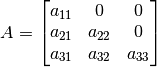
The linear equation is the most elementary problem that arises in computational economic analysis. In a linear equation, an  matrix
  and an n-vector
  are given, and one must compute the
  -vector
  that satisfies
  .
.
Linear equations arise naturally in many economic applications such as
Linear multicommodity market equilibrium models
Finite-state financial market models
Markov chain models
Ordinary least squares
They more commonly arise indirectly from numerical solution to nonlinear and functional equations:
Nonlinear multicommodity market models
Multiperson static game models
Dynamic optimization models
Rational expectations models
Applications often require the repeated solution of very large linear equation systems. In these situations, issues regarding speed, storage requirements, and preciseness of the solution of such equations can arise.
[1]:
import pandas as pd
import numpy as np

from linear_algorithms import backward_substitution
from linear_algorithms import forward_substitution
from linear_algorithms import gauss_seidel
from linear_algorithms import solve

from linear_plots import plot_operation_count

from temfpy.linear_equations import get_ill_cond_lin_eq
from linear_problems import get_inverse_demand_problem
Special cases
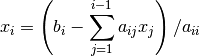
We can start with some special cases to develop a basic understanding for the core building blocks for more complicated settings. Let’s start with the case of a lower triangular matrix , where we can solve the linear equation by a simple backward or forward substitution. Let’s consider the following setup.
Consider an algorithmic implementation of forward-substitution as an example.
[2]:
??forward_substitution
[3]:
def test_problem():
    A = np.tril(np.random.normal(size=(3, 3)))
    x = np.random.normal(size=3)
    b = np.matmul(A, x)
    return A, b, x


for _ in range(10):
    A, b, x_true = test_problem()
    x_solve = forward_substitution(A, b)
    np.testing.assert_almost_equal(x_solve, x_true)
Questions
How can we make the test code more generic and sample test problems of different dimensions?
Is there a way to control the randomness in the test function?
Is there software out there that allows to automate parts of the testing?
If we have an upper triangular matrix, we can use backward substitution to solve the linear system
[4]:
??backward_substitution
Exercise
Implement the same testing setup as above the backward-substitution function.
We can now build on these two functions to tackle more complex tasks. This is a good example on how to develop scientific software step-by-step ensuring that each component is well tested before integrating into more involved settings.
L-U Factorization
Most linear equations encountered in practice, however, do not have a triangular matrix. Doolittle and Crout have shown that any matrix can be decomposed into the product of a (row-permuted) lower and upper triangular matrix  and
and  , respectively
  using Gaussian elimination. We will not look into the Gaussian elimination algorithm, but there is an example application in our textbook where you can follow along step by step. The L-U
algorithm is designed to decompose the matrix into the product of lower and upper triangular matrices, allowing the linear equation to be solved using a combination of backward and forward substitution.
using Gaussian elimination. We will not look into the Gaussian elimination algorithm, but there is an example application in our textbook where you can follow along step by step. The L-U
algorithm is designed to decompose the matrix into the product of lower and upper triangular matrices, allowing the linear equation to be solved using a combination of backward and forward substitution.
Here are the two core steps:
Factorization phase

Solution phase:

where we solve  using forward-substitution and
  using backward-substitution.
Adding to this the two building blocks we developed earlier forward_substitution and backward_substitution, we can now write a quite generic function to solve systems of linear equations.
[5]:
??solve
Let’s see if this is actually working.
[6]:
A = np.array([[3, 1], [1, 2]])
x_true = np.array([9, 8])
b = A @ x_true
x_solve = solve(A, b)
np.testing.assert_almost_equal(x_true, x_solve)
Pivoting
Rounding error can cause serious error when solving linear equations. Let’s consider the following example, where  is a tiny number.
![\begin{bmatrix} \epsilon & 1\\ 1 & 1 \end{bmatrix} \times \left[ \begin{array}{c} x_1 \\ x_2 \end{array} \right] = \left[\begin{array}{c} 1 \\ 2 \end{array} \right]](../../_images/math/79be0678f04ae15f833d9f89f86f81652c1cbbec.png)
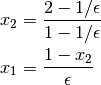
It is easy to verify that the right solution is

and thus  is slightly more than one and
  is slightly less than one. To solve the system using Gaussian elimination we need to add
  times the first row to the second row. We end up with
![\begin{bmatrix} \epsilon & 1 \\ 0 & 1 - \frac{1}{\epsilon} \end{bmatrix} \times \left[ \begin{array}{c} x_1 \\ x_2 \end{array} \right] = \left[ \begin{array}{c} 1 \\ 2 - \frac{1}{\epsilon} \end{array} \right],](../../_images/math/b9bfb44e1b7417d225e9ff81eaeb27924adefc0a.png)
which we can then solve recursively.
Let’s translate this into code.
[7]:
eps = 1e-17
A = np.array([[eps, 1], [1, 1]])
b = np.array([1, 2])
We can now use our solution algorithm.
[8]:
solve(A, b)
[8]:
array([0., 1.])
But we have to realize that the results are grossly inaccurate. What happened? Is there any hope to apply numpy’s routine?
[9]:
np.linalg.solve(A, b)
[9]:
array([1., 1.])
This algorithm does automatically check whether such rounding errors can be avoided by simply changing the order of rows. This is called pivoting and changes the recursive solution to

which can be solved more accurately. Our implementation also solves the modified problem well.
[10]:
A = np.array([[1, 1], [eps, 1]])
b = np.array([2, 1])
solve(A, b)
[10]:
array([1., 1.])
Building your own numerical routines is usually the only way to really understand the algorithms and learn about all the potential pitfalls. However, the default should be to rely on battle-tested production code. For linear algebra there are numerous well established libraries available. Building your own numerical routines is usually the only way to really understand the algorithms and learn about all the potential pitfalls. However, the default should be to rely on battle-tested production code. For linear algebra there are numerous well established libraries available.
Benchmarking
How does solving a system of linear equations by an  decomposition compare to other alternatives of solving the system of linear equations.
[11]:
plot_operation_count()
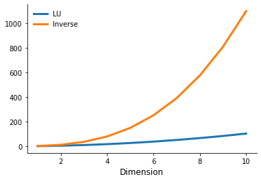
The right setup for your numerical needs depends on your particular problem. For example, this trade-off looks very different if you have to solve numerous linear equations that only differ in but not . In this case you only need to compute the inverse once.
Exercise
Set up a benchmarking exercise that compares the time to solution for the two approaches for
 and
and  , where denotes the number of linear equations and
  the number of repeated solutions.
Ill Conditioning
Some linear equations are inherently difficult to solve accurately on a computer. This difficulty occurs when the A matrix is structured in such a way that a small perturbation  in the data vector induces a large change
  in the solution vector . In such cases the linear equation or, more generally, the matrix is said to be ill conditioned.
One measure of ill conditioning in a linear equation Ax = b is the “elasticity” of the solution vector with respect to the data vector
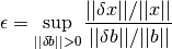
The elasticity gives the maximum percentage change in the size of the solution vector induced by a  percent change in the size of the data vector . If the elasticity is large, then small errors in the computer representation of the data vector can produce large errors in the computed solution vector x. Equivalently, the computed solution will have far fewer significant digits than the data vector .
In practice, the elasticity is estimated using the condition number of the matrix , which for invertible is defined by 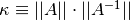 . The condition number is always greater than or equal to one. Numerical analysts often use the rough rule of thumb that for each power of
  in the condition number, one significant digit is lost in the computed solution vector . Thus, if has a condition number of
  , the
computed solution vector will have about three fewer significant digits than the data vector .
, the
computed solution vector will have about three fewer significant digits than the data vector .
Let’s look at an example, where the solution vector is all ones but but the linear equation is notoriously ill-conditioned.
[12]:
??get_ill_cond_lin_eq
How does the solution error depend on the condition number in this setting.
[13]:
rslt = dict((("Condition", []), ("Error", []), ("Dimension", [])))
grid = [5, 10, 15, 25]

for n in grid:
    A, b, x_true = get_ill_cond_lin_eq(n)
    x_solve = np.linalg.solve(A, b)
    rslt["Condition"].append(np.linalg.cond(A))
    rslt["Error"].append(np.linalg.norm(x_solve - x_true, 1))
    rslt["Dimension"].append(n)
[14]:
pd.DataFrame.from_dict(rslt)
[14]:
| Condition | Error | Dimension | |
|---|---|---|---|
| 0 | 2.616969e+04 | 1.278000e+03 | 5 |
| 1 | 2.106258e+12 | 1.762345e+09 | 10 |
| 2 | 2.582411e+21 | 4.947153e+16 | 15 |
| 3 | 2.035776e+22 | 2.383979e+20 | 25 |
There is a more general lesson here. Always be skeptical about the quality of your numerical results. See these two papers for an exploratory analysis of econometric software packages and nonliner optimization. Yes, they are rather old and much progress has been made, but the general points remain valid.
McCullough, B. D., and Vinod, H. D. (2003). Verifying the Solution from a Nonlinear Solver: A Case Study. American Economic Review, 93 (3): 873-892.
McCullough, B., D., and Vinod H. D. (1999). The Numerical Reliability of Econometric Software. Journal of Economic Literature, 37 (2): 633-665.
Exercise
Let’s consider the following example as well, which is taken from Johansson (2015, p.131).
![\left[\begin{array}{c} 1 \\ 2 \end{array}\right] = \begin{bmatrix} 1 & \sqrt{p}\\ 1 & \frac{1}{\sqrt{p}} \end{bmatrix} \times \left[ \begin{array}{c} x_1 \\ x_2 \end{array} \right]](../../_images/math/6baa273eee4c8fdeef1659a87c7e22aa1aff38ee.png)
This system is singular for  and for
  in the vicinity of one is ill-conditioned.
Create two plots that show the condition number and the error between the analytic and numerical solution.
Iterative methods
Algorithms based on Gaussian elimination are called exact or, more properly, direct methods because they would generate exact solutions for the linear equation after a finite number of operations, if not for rounding error. Such methods are ideal for moderately sized linear equations but may be impractical for large ones. Other methods, called iterative methods, can often be used to solve large linear equations more efficiently if the matrix is sparse, that is, if
is composed mostly of zero entries. Iterative methods are designed to generate a sequence of increasingly accurate approximations to the solution of a linear equation, but they generally do not yield an exact solution after a prescribed number of steps, even in theory.
The most widely used iterative methods for solving a linear equation are developed by choosing an easily invertible matrix  and writing the linear equation in the equivalent form
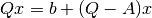
or
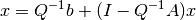
This form of the linear equation suggests the iteration rule

which, if convergent, must converge to a solution of the linear equation. Ideally, the so-called splitting matrix will satisfy two criteria. First,  and
and  should be relatively easy to compute. This criterion is met if is either diagonal or triangular. There are two popular approaches:
The Gauss-Seidel method sets
equal to the upper triangular matrix formed from the upper triangular elements of .The Gauss-Jacobi method sets
equal to the diagonal matrix formed from the diagonal entries of .
[15]:
??gauss_seidel
Exercise
Implement the Gauss-Jacobi method.
[16]:
from linear_solutions_tests import gauss_jacobi # noqa: E402
Let’s conclude with an economic application as outlined in Judd (1998). Suppose we have the following inverse demand function  and the following supply curve
  . Equilibrium is where supply equals demand and thus we need to solve the following linear system.
![\left[\begin{array}{c} 10 \\ -2 \end{array}\right] = \begin{bmatrix} 1 & 1\\ 1 & -2\end{bmatrix} \times \left[ \begin{array}{c} p \\ q \end{array} \right]](../../_images/math/e491addd1c0d30872778bb24c687ffed3b658f4a.png)
[17]:
A, b, x_true = get_inverse_demand_problem()
Now we can compre the two solution approaches and make sure that they in fact give the same result.
[18]:
x_seidel = gauss_seidel(A, b)
x_jacobi = gauss_jacobi(A, b)
np.testing.assert_almost_equal(x_seidel, x_jacobi)
Resources
The PARDISO Solver Project: https://www.pardiso-project.org
LAPACK — Linear Algebra PACKage: http://www.netlib.org/lapack
Robert Johansson. Numerical Python: scientific computing and data science applications with NumPy, SciPy and Matplotlib. Apress, 2018.
William H Press, Brian P Flannery, Saul A Teukolsky, and William T Vetterling. Numerical recipes: The art of scientific computing. Cambridge University Press, 1986.
[ ]: