Download the notebook here!
Interactive online version: ![]()
Optimization
[1]:
from functools import partial
from temfpy.optimization import carlberg

from scipy import optimize as opt
import matplotlib.pyplot as plt
from scipy.stats import norm
import seaborn as sns
import scipy as sp
import pandas as pd
import numpy as np

from optimization_problems import get_test_function_gradient
from optimization_problems import get_parameterization
from optimization_problems import get_test_function
from optimization_auxiliary import process_results
from optimization_auxiliary import get_bounds
from optimization_plots import plot_contour
from optimization_plots import plot_surf
from optimization_plots import plot_optima_example
from optimization_plots import plot_true_observed_example
Outline
Setup
Algorithms
Gradient-based methods
Derivative-free methods
Benchmarking exercise
Special cases
Setup
In the finite-dimensional unconstrained optimization problem, one is given a function  and asked to find an
  such that
  for all
  . We call
  the objective function and , if it exists, the global minimum of . We focus on minimum - to solve a minimization problem, simply minimize the negative of the objective.
We say that  is a …
strict global minimum of
if  for all
  .
.weak local minimum of
if  for all in some neighborhood of .
strict local minimum of
if  for all in some neighborhood of .
[2]:
plot_optima_example()
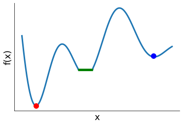
Let  be twice continuously differentiable.
First Order Necessary Conditions: If
is a local minimum of , then  .
.Second Order Necessary Condition: If
is a local minimum of , then  is negative semidefinite.
We say is a critical point of if it satisfies the first-order necessary condition.
Sufficient Condition: If
 and
and  is negative definite, then is a strict local minimum of .
Local-Global Theorem: If
is concave, and is a local minimum of , then is a global minimum of .
Key problem attributes
Convexity: convex vs. non-convex
Optimization-variable type: continuous vs. discrete
Constraints: unconstraint vs. constraint
Number of optimization variables: low-dimensional vs. high-dimensional
These attributes dictate:
ability to find solution
problem complexity and computing time
appropriate methods
relevant software
 Always begin by categorizing your problem
Optimization problems are ubiquitous in economics:
Government maximizes social welfare
Competitive equilibrium maximizes total surplus
Ordinary least squares estimator minimizes sum of squares
Maximum likelihood estimator maximizes likelihood function
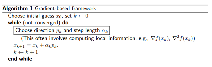
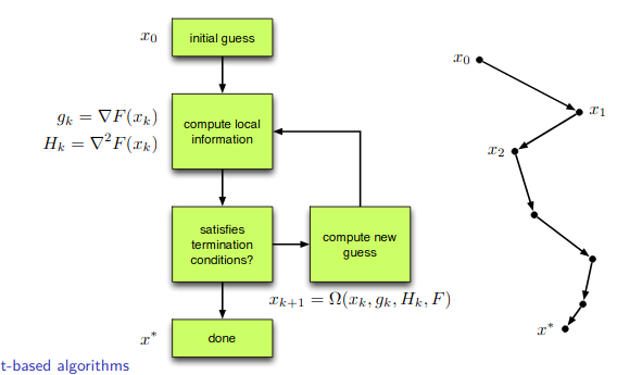
Algorithms
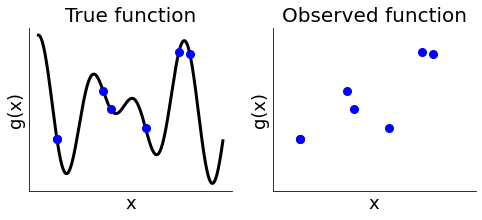
We are mostly blind to the function we are trying to minimize and can only compute the function at a limited number of points. Each evaluation is computationally expensive.
[3]:
plot_true_observed_example()
Goals
reasonable memory requirements
low failure rate, convergence conditions are met
convergence in a few iterations with low cost for each iteration
Catergorization
gradient-based vs. derivative-free
global vs. local
Question
How to compute derivatives?
Gradient-based methods
Benefits
efficient for many variables
well-suited for smooth objective and constraint functions
Drawbacks
requires computing the gradient, potentially challenging and time-consuming
convergence is only local
not-well suited for noisy functions, derivative information flawed
Second derivative are also very useful, but …
Hessians are
 , so expensive to construct and store
often only approximated using quasi-Newton methods
Questions
How to use gradient-based algorithms to find a global optimum?
Any ideas on how to reduce the memory requirements for a large Hessian?
There is two different classes of gradient-based algorithms.
Line-search methods
compute
 be a descent direction
compute
 to produce a sufficient decrease in the objective function
Let’s see here for how such a line search looks like in practice for the Newton-CG algorithm.
Trust-region methods
determine a maximum allowable step length (trust-region radius)

compute step
 with
with  using a model
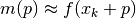
As an example implementation, see here for the scipy.optimize_trustregion.py implementation.
Derivative-Free Methods
Benefits
often better at finding a global minimum if function not convex
robust with respect to noise in criterion function
amenable to parallelization
Drawbacks
extremely slow convergence for high-dimensional problems
There are two different classes of derivative-free algorithms.
heuristic, inspired by nature
basin-hopping
evolutionary algorithms
direct search
directional
simplicial
Test function
![f(x) = \tfrac{1}{2}\sum_{i=1}^n a_i\cdot (x_i-1)^2+ b\cdot \left[ n-\sum_{i=1}^n\cos(2\pi(x_i-1))\right],](../../_images/math/3f249a97418d36813afac1603cf0e1b5c2fae993.png)
where  and
and  provide the parameterization of the function.
Exercises
Implement this test function.
Visualize the shape of our test function for the one-dimensional case.
What is the role of the parameters
 and ?
and ?What is the functions global minimum?
[4]:
??get_test_function
[5]:
??get_parameterization
We want to be able to use our test function for different configurations of the challenges introduced by noise and ill-conditioning.
[6]:
add_noise, add_illco, x0 = False, False, [4.5, -1.5]


def get_problem(dimension, add_noise, add_illco, seed=123):
    np.random.seed(seed)
    a, b = get_parameterization(dimension, add_noise, add_illco)
    get_test_function_p = partial(get_test_function, a=a, b=b)
    get_test_function_gradient_p = partial(get_test_function_gradient, a=a, b=b)
    return get_test_function_p, get_test_function_gradient_p


dimension = len(x0)
opt_test_function, opt_test_gradient = get_problem(dimension, add_noise, add_illco)
np.testing.assert_equal(opt_test_function([1, 1]), 0.0)
Let’s see how the surface and contour plots look like under different scenarios.
[7]:
opt_test_function, _ = get_problem(dimension, add_noise, add_illco)
plot_surf(opt_test_function)
/Users/emilyschwab/Desktop/IAME_Work/ose-course-scientific-computing/labs/optimization/optimization_plots.py:62: MatplotlibDeprecationWarning: Calling gca() with keyword arguments was deprecated in Matplotlib 3.4. Starting two minor releases later, gca() will take no keyword arguments. The gca() function should only be used to get the current axes, or if no axes exist, create new axes with default keyword arguments. To create a new axes with non-default arguments, use plt.axes() or plt.subplot().
  ax = fig.gca(projection="3d")
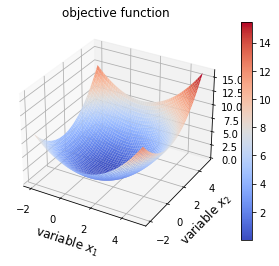
Question
How is the global minimum affected by the addition of noise and ill-conditioning?
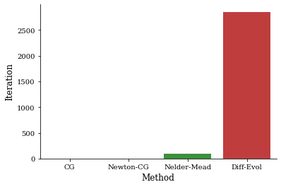
Benchmarking exercise
Let’s get our problem setting and initialize a container for our results. We will use the convenient interface to scipy.optimize.minimize. Its documentation also points you to research papers and textbooks where the details of the algorithms are discussed in more detail. We need to invest a little in the design of our setup first, but then we can run the benchmarking exercise with ease and even adding additional optimization algorithms is straightforward.
[8]:
ALGORITHMS = ["CG", "Newton-CG", "Nelder-Mead", "Diff-Evol"]
add_noise, add_illco, dimension = False, False, 2
[9]:
x0 = [4.5, -1.5]
opt_test_function, opt_test_gradient = get_problem(dimension, add_noise, add_illco)
df = pd.DataFrame(columns=["Iteration", "Distance"], index=ALGORITHMS)
df.index.name = "Method"
Let’s fix what will stay unchanged throughout.
[10]:
call_optimizer = partial(
    opt.minimize,
    fun=opt_test_function,
    x0=x0,
    jac=opt_test_gradient,
    options={"disp": True, "return_all": True, "maxiter": 100000},
)
We prepared some functions to process results from the optimizer calls.
[11]:
??process_results
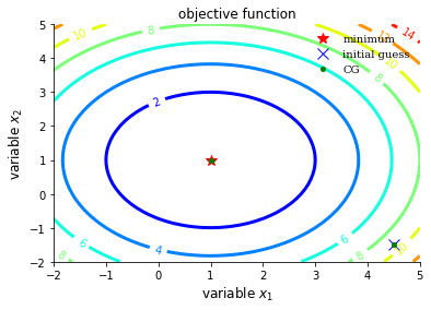
Conjugate gradient
[12]:
method = "CG"
res = call_optimizer(method=method)
initial_guess = [4.5, -1.5]
df = process_results(df, method, res)
plot_contour(opt_test_function, res["allvecs"], method, initial_guess)
Optimization terminated successfully.
         Current function value: 0.000000
         Iterations: 1
         Function evaluations: 3
         Gradient evaluations: 3
[12]:
<module 'matplotlib.pyplot' from '/Users/emilyschwab/miniconda3/envs/ose-course-scientific-computing/lib/python3.8/site-packages/matplotlib/pyplot.py'>
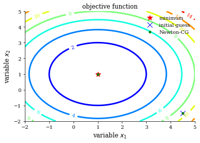
Newton-CG
[13]:
method = "Newton-CG"
res = call_optimizer(method=method)
initial_guess = [4.5, -1.5]
df = process_results(df, method, res)
plot_contour(opt_test_function, res["allvecs"], method, initial_guess)
Optimization terminated successfully.
         Current function value: 0.000000
         Iterations: 2
         Function evaluations: 2
         Gradient evaluations: 3
         Hessian evaluations: 0
[13]:
<module 'matplotlib.pyplot' from '/Users/emilyschwab/miniconda3/envs/ose-course-scientific-computing/lib/python3.8/site-packages/matplotlib/pyplot.py'>
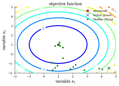
Nelder Mead
[14]:
method = "Nelder-Mead"
res = call_optimizer(method=method)
initial_guess = [4.5, -1.5]
df = process_results(df, method, res)
plot_contour(opt_test_function, res["allvecs"], method, initial_guess)
Optimization terminated successfully.
         Current function value: 0.000000
         Iterations: 51
         Function evaluations: 95
/Users/emilyschwab/miniconda3/envs/ose-course-scientific-computing/lib/python3.8/site-packages/scipy/optimize/_minimize.py:522: RuntimeWarning: Method Nelder-Mead does not use gradient information (jac).
  warn('Method %s does not use gradient information (jac).' % method,
[14]:
<module 'matplotlib.pyplot' from '/Users/emilyschwab/miniconda3/envs/ose-course-scientific-computing/lib/python3.8/site-packages/matplotlib/pyplot.py'>
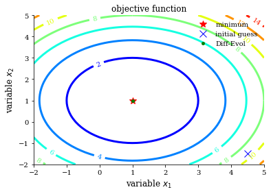
Differential evolution
[15]:
??get_bounds
[16]:
method = "Diff-Evol"
res = opt.differential_evolution(opt_test_function, get_bounds(dimension))
initial_guess = [4.5, -1.5]
plot_contour(opt_test_function, res["x"], method, initial_guess)
df = process_results(df, method, res)
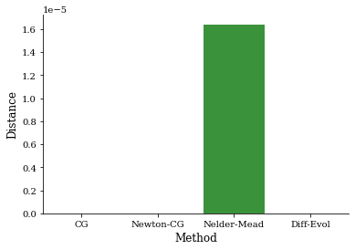
Summary
[17]:
_ = sns.barplot(x="Method", y="Iteration", data=df.reset_index())
[18]:
_ = sns.barplot(x="Method", y="Distance", data=df.reset_index())
Speeding up test function
We want to increase the dimensionality of our optimization problem going forward. Even in this easy setting, it is worth to re-write our objective function using numpy to ensure its speedy execution. A faster version is already available as part of the Python package temfpy. Below, we compare our test function to the temfpy version and assess their performance in regard to speed.
[19]:
??get_test_function
[20]:
??carlberg
It is very easy to introduce errors when speeding up your code as usually you face a trade-off between readability and performance. However, setting up a simple testing harness that simply compares the results between the slow, but readable, implementation and the fast one for numerous random test problems. For more automated, but random, testing see Hypothesis.
[21]:
def get_speed_test_problem():
    add_illco, add_noise = np.random.choice([True, False], size=2)
    dimension = np.random.randint(2, 100)

    a, b = get_parameterization(dimension, add_noise, add_illco)
    x0 = np.random.uniform(size=dimension)
    return x0, a, b
Now we are ready to put our fears at ease.
[22]:
for _ in range(1000):
    args = get_speed_test_problem()
    stats = get_test_function(*args), carlberg(*args)
    np.testing.assert_almost_equal(*stats)
Let’s see whether this was worth the effort for a small and a large problem using the %timeit magic function.
[23]:
dimension, add_noise, add_illco = 100, True, True
x0 = np.random.uniform(size=dimension)
a, b = get_parameterization(dimension, add_noise, add_illco)
[24]:
%timeit carlberg(x0, a, b)
51.6 µs ± 20.3 µs per loop (mean ± std. dev. of 7 runs, 10000 loops each)
[25]:
%timeit get_test_function(x0, a, b)
618 µs ± 198 µs per loop (mean ± std. dev. of 7 runs, 1000 loops each)
In this particular setting, there is no need to increase the performance even further. However, as a next step, check out numba, for even more flexibility in speeding up your code.
Exercises
Repeat the exercise in the case of noise in the criterion function and try to summarize your findings.
What additional problems arise as the dimensionality of the problem for a 100-dimensional problem? Make sure to use the fast implementation of the test function.
Special cases
Nonlinear least squares and maximum likelihood estimation have special structure that can be exploited to improve the approximation of the inverse Hessian.
Nonlinear least squares
We will estimate the following nonlinear consumption function using data from Greene’s textbook:
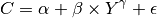
which is estimated with quarterly data on real consumption and disposable income for the U.S. economy from 1950 to 2000.
[26]:
df = pd.read_pickle("material/data-consumption-function.pkl")
df.head()
[26]:
| realgdp | realcons | ||
|---|---|---|---|
| Year | qtr | ||
| 1950 | 1 | 1610.5 | 1058.9 |
| 2 | 1658.8 | 1075.9 | |
| 3 | 1723.0 | 1131.0 | |
| 4 | 1753.9 | 1097.6 | |
| 1951 | 1 | 1773.5 | 1122.8 |
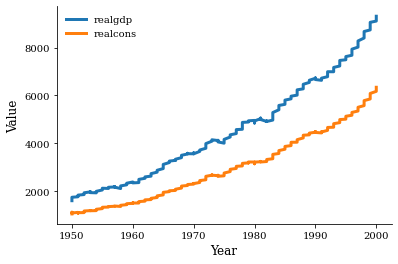
Let’s confirm the basic relationship to get an idea of what to expect for the estimated parameters.
[27]:
fig, ax = plt.subplots()
x = df.index.get_level_values("Year")

for name in ["realgdp", "realcons"]:
    y = df[name]
    ax.plot(x, y, label=name)

ax.set_xlabel("Year")
ax.set_ylabel("Value")
ax.legend()
[27]:
<matplotlib.legend.Legend at 0x11dc95c70>
Now we set up the criterion function such that it fits the requirements.
[28]:
consumption = df["realcons"].values
income = df["realgdp"].values


def ssr(x, consumption, income):
    alpha, beta, gamma = x
    residuals = consumption - alpha - beta * income ** gamma
    return residuals


ssr_partial = partial(ssr, consumption=consumption, income=income)
rslt = sp.optimize.least_squares(ssr_partial, [0, 0, 1])["x"]
Exercise
Evaluate the fit of the model.
Maximum likelihood estimation
Greene (2012) considers the following binary choice model.
![\begin{align*}
P[Grade = 1] = F(\beta_0 + \beta_1 GPA + \beta_2 TUCE + \beta_3 PSI)
\end{align*}](../../_images/math/bd0bf50aa315319ab351c036beee1701dba00b26.png)
where  the cumulative distribution function for either the normal distribution (Probit) or the logistic distribution (Logit).
[29]:
df = pd.read_pickle("material/data-graduation-prediction.pkl")
df.head()
[29]:
| GPA | TUCE | PSI | GRADE | INTERCEPT | GRADE | |
|---|---|---|---|---|---|---|
| OBS | ||||||
| 1 | 2.66 | 20 | 0 | 0 | 1 | 0 |
| 2 | 2.89 | 22 | 0 | 0 | 1 | 0 |
| 3 | 3.28 | 24 | 0 | 0 | 1 | 0 |
| 4 | 2.92 | 12 | 0 | 0 | 1 | 0 |
| 5 | 4.00 | 21 | 0 | 1 | 1 | 1 |
[30]:
def probit_model(beta, y, x):
    F = norm.cdf(x @ beta)
    fval = (y * np.log(F) + (1 - y) * np.log(1 - F)).sum()
    return -fval
[31]:
x, y = df[["INTERCEPT", "GPA", "TUCE", "PSI"]], df["GRADE"]
rslt = opt.minimize(probit_model, [0.0] * 4, args=(y, x))
Exercise
Amend the code so that you can simply switch between estimating a Probit or Logit model.
Resources
Kevin T. Carlberg: https://kevintcarlberg.net
Software
SNOPT (Sparse Nonlinear OPTimizer): https://ccom.ucsd.edu/~optimizers/solvers/snopt
Gurobi https://www.gurobi.com
IBM CPLEX Optimizer https://www.ibm.com/analytics/cplex-optimizer
Books
Nocedal, J., & Wright, S. (2006). *Numerical optimization* . Springer Science & Business Media.
Boyd, S., Boyd, S. P., & Vandenberghe, L. (2004). *Convex optimization*. Cambridge university press.
Kochenderfer, M. J., & Wheeler, T. A. (2019). *Algorithms for optimization*. Mit Press.
Fletcher, R. (2000). *Practical methods of optimization (2nd edn)*. Wiley.
Nesterov, Y. (2018). *Lectures on convex optimization*. Springer Nature Switzerland.
Research
Moré, J. J., & Wild, S. M. (2009). Benchmarking derivative-free optimization algorithms. SIAM Journal on Optimization, 20(1), 172-191.
Beiranvand, V., Hare, W., & Lucet, Y. (2017). Best practices for comparing optimization algorithms. Optimization and Engineering, 18, 815–848.
Bartz-Beielstein, T., et al. (2020). Benchmarking in optimization: Best practice and open issues. arXiv preprint arXiv:2007.03488..