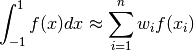
Download the notebook here!
Interactive online version: ![]()
Integration
[1]:
import numpy as np

from integration_algorithms import monte_carlo_quasi_two_dimensions
from integration_algorithms import quadrature_newton_trapezoid_one
from integration_algorithms import quadrature_newton_simpson_one
from integration_algorithms import quadrature_gauss_legendre_one
from integration_algorithms import quadrature_gauss_legendre_two
from integration_algorithms import monte_carlo_naive_one

from integration_plots import plot_naive_monte_carlo_randomness
from integration_plots import plot_naive_monte_carlo_error
from integration_plots import plot_gauss_legendre_weights
from integration_plots import plot_benchmarking_exercise
from integration_plots import plot_naive_monte_carlo
from integration_plots import plot_quasi_monte_carlo
from integration_plots import plot_starting_illustration
from integration_plots import plot_trapezoid_rule_illustration
from integration_plots import plot_simpsons_rule_illustration

from integration_problems import problem_kinked
from integration_problems import problem_smooth
Outline
Setup
Newton-Cotes rules
Gaussian formulas
Monte Carlo integration
Resources
Setup
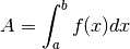
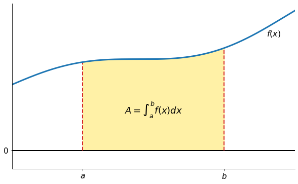
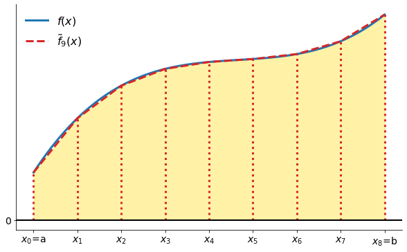
Consider finding the area under a continuous real-valued function  over a bounded interval
 ![[a, b]](../../_images/math/e219413cc39d1f0e877b563af388435f55f73b68.png) :
:
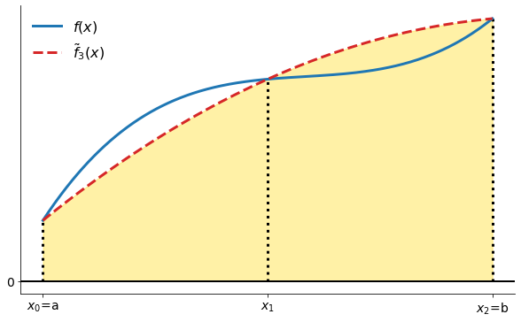
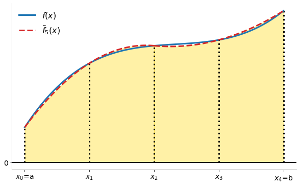
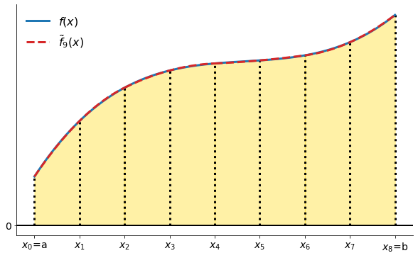
Let’s look a visual representation of our problem.
[2]:
plot_starting_illustration()
Most numerical methods for computing this integral split up the original integral into a sum of several integrals, each covering a smaller part of the original integration interval . This re-writing of the integral is based on a selection of integration points  that are distributed on the interval . Integration points may, or may not, be evenly distributed.
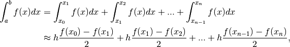
Given the integration points, the original integral is re-written as a sum of integrals, each integral being computed over the sub-interval between two consecutive integration points. The integral from the beginning is thus expressed as:
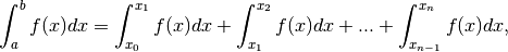
where  and
and  .
.
The different integration methods will differ in the way they approximate each integral on the right hand side. The fundamental idea is that each term is an integral over a small interval ![[x_i , x_{i+1}]](../../_images/math/dd5489e165288e0f11acb66caa99a6a6409c68f9.png) , and over this small interval, it makes sense to approximate by a simple shape
, and over this small interval, it makes sense to approximate by a simple shape
Newton-Cotes rules
Newton–Cotes quadrature rules are a group of formulas for numerical integration (also called quadrature) based on evaluating the integrand at equally spaced points. The integration points are then computed as

where 
The closed Newton-Cotes formula of degree  is stated as
We will consider the first two degrees in more detail:
Trapezoid rule
Simpson’s rule
Trapezoid rule
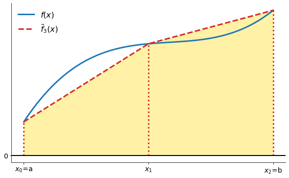
The Trapezoid rule approximates the area under the function with the area under a piecewise linear approximation to .
[3]:
plot_trapezoid_rule_illustration()
More formally:
which we can further simplify to:
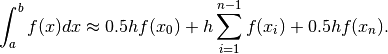
The weights are then the following:
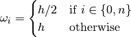
[4]:
??quadrature_newton_trapezoid_one
Signature: quadrature_newton_trapezoid_one(f, a, b, n)
Source:
def quadrature_newton_trapezoid_one(f, a, b, n):
    """Return quadrature newton trapezoid example."""
    xvals = np.linspace(a, b, n + 1)
    fvals = np.tile(np.nan, n + 1)
    h = xvals[1] - xvals[0]

    weights = np.tile(h, n + 1)
    weights[0] = weights[-1] = 0.5 * h

    for i, xval in enumerate(xvals):
        fvals[i] = f(xval)

    return np.sum(weights * fvals)
File:      ~/external-storage/sciebo/office/OpenSourceEconomics/teaching/scientific-computing/course/lectures/integration/integration_algorithms.py
Type:      function
[5]:
integrand = quadrature_newton_trapezoid_one(np.exp, 0, 1, 1000)
np.testing.assert_almost_equal(integrand, np.exp(1) - 1)
Simpson’s rule
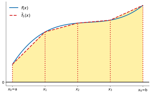
Simpson’s rule approximates the area under a function with the area under a piecewise quadratic approximation to .
[6]:
plot_simpsons_rule_illustration()
The weights are the following:
![\begin{aligned}
w_i = \begin{cases}
h / 3 & \text{for $i \in [0, n]$} \\
4 h / 3& \text{for $0 < i < n, i$ even} \\
2 h / 3& \text{for $0 < i < n, i$ odd} . \\
\end{cases}
\end{aligned}](../../_images/math/49056ad2b44028fda3d170234f633889a0763d99.png)
[7]:
??quadrature_newton_simpson_one
Signature: quadrature_newton_simpson_one(f, a, b, n)
Source:
def quadrature_newton_simpson_one(f, a, b, n):
    """Return quadrature newton simpson example."""
    if n % 2 == 0:
        raise Warning("n must be an odd integer. Increasing by 1")
        n += 1

    xvals = np.linspace(a, b, n)
    fvals = np.tile(np.nan, n)

    h = xvals[1] - xvals[0]

    weights = np.tile(np.nan, n)
    weights[0::2] = 2 * h / 3
    weights[1::2] = 4 * h / 3
    weights[0] = weights[-1] = h / 3

    for i, xval in enumerate(xvals):
        fvals[i] = f(xval)

    return np.sum(weights * fvals)
File:      ~/external-storage/sciebo/office/OpenSourceEconomics/teaching/scientific-computing/course/lectures/integration/integration_algorithms.py
Type:      function
[8]:
integrand = quadrature_newton_simpson_one(np.exp, 0, 1, 1001)
np.testing.assert_almost_equal(integrand, np.exp(1) - 1)
Gaussian formulas
Gaussian quadrature formulas employ a very different logic to compute the area under a curve over a bounded interval . Specifically, the quadrature nodes  and quadrature weights
  are chosen to exactly integrate polynomials of degree
  or less.
Gaussian quadrature approximations of the form:
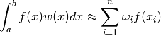
for any nonnegative weighing function  . Versions of lead to include Gauss-Legendre, Gauss-Chebyshev, Gauss-Hermite and Gauss-Laguerre.
We start from the special domain between ![[-1, 1]](../../_images/math/92b4b754966e4a581f924d4bfd1b0db7ab47c886.png) , again the formula for our approximate solution looks very similar.
, again the formula for our approximate solution looks very similar.
So, more generally using a change of variables:
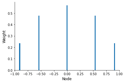
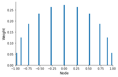
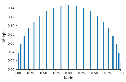
Unlike in the case of the Newton-Cotes approach, Gaussian nodes are not uniformly spaced and do not include the integration limits.
[9]:
[plot_gauss_legendre_weights(deg) for deg in [5, 11, 21]]
[9]:
[None, None, None]
Question
What are the properties of the weights?
[10]:
??quadrature_gauss_legendre_one
Signature: quadrature_gauss_legendre_one(f, a, b, n)
Source:
def quadrature_gauss_legendre_one(f, a, b, n):
    """Return quadrature gauss legendre example."""
    xvals, weights = np.polynomial.legendre.leggauss(n)
    xval_trans = (b - a) * (xvals + 1.0) / 2.0 + a

    fvals = np.tile(np.nan, n)
    for i, xval in enumerate(xval_trans):
        fvals[i] = ((b - a) / 2.0) * f(xval)

    return np.sum(weights * fvals)
File:      ~/external-storage/sciebo/office/OpenSourceEconomics/teaching/scientific-computing/course/lectures/integration/integration_algorithms.py
Type:      function
[11]:
integrand = quadrature_gauss_legendre_one(np.exp, 0, 1, 1000)
np.testing.assert_almost_equal(integrand, np.exp(1) - 1)
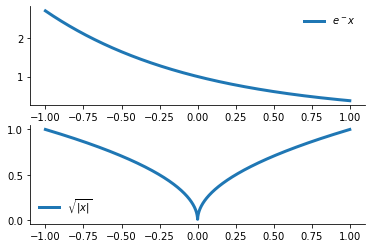
Benchmarking
Exercise
Compare the performance of our integration routines on the following two integrals.
We study the following two cases:
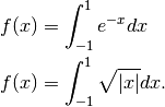
[12]:
plot_benchmarking_exercise()
How can we extend the ideas so far to multidimensional integration?
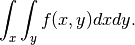
The product rule approximates the integral with the following sum:
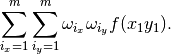
A difficulty of this approach is the curse of dimensionality as the number of nodes inreases exponentially with the number of dimensions.
[13]:
??quadrature_gauss_legendre_two
Signature: quadrature_gauss_legendre_two(f, a=-1, b=1, n=10)
Source:
def quadrature_gauss_legendre_two(f, a=-1, b=1, n=10):
    """Return quadrature gauss legendre example."""
    n_dim = int(np.sqrt(n))

    xvals, weight_uni = np.polynomial.legendre.leggauss(n_dim)
    xvals_transformed = (b - a) * (xvals + 1.0) / 2.0 + a

    weights = np.tile(np.nan, n_dim ** 2)
    fvals = np.tile(np.nan, n_dim ** 2)

    counter = 0
    for i, x in enumerate(xvals_transformed):
        for j, y in enumerate(xvals_transformed):
            weights[counter] = weight_uni[i] * weight_uni[j]
            fvals[counter] = f([x, y])
            counter += 1

    return ((b - a) / 2) ** 2 * np.sum(weights * np.array(fvals))
File:      ~/external-storage/sciebo/office/OpenSourceEconomics/teaching/scientific-computing/course/lectures/integration/integration_algorithms.py
Type:      function
Monte Carlo integration
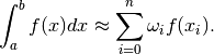
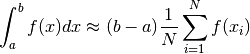
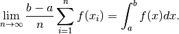
Naive Monte Carlo integration uses random sampling of a function to numerically compute an estimate of its integral. We can approximate this integral by averaging  samples of the function drawn from a uniform distribution between
  and
and  .
.
Why?
![\begin{aligned}
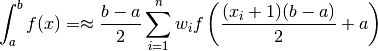
E\left[ (b - a) \frac{1}{N} \sum_{i = 1}^N f(x_i)\right] & = (b - a) \frac{1}{N} \sum_{i = 1}^N E\left[f(x_i)\right] \\
& = (b - a) \frac{1}{N} \sum_{i = 1}^N\left[\int_a^b f(x) \frac{1}{b - a} dx\right] \\
& = \frac{1}{N} \sum_{i = 1}^N \int_a^b f(x) dx \\
& = \int_a^b f(x) dx.
\end{aligned}](../../_images/math/b5c2e4885e8693a7f75f89e42eb7e939821c5f15.png)
[14]:
??monte_carlo_naive_one
Signature: monte_carlo_naive_one(f, a=0, b=1, n=10, seed=123)
Source:
def monte_carlo_naive_one(f, a=0, b=1, n=10, seed=123):
    """Return naive monte carlo example."""
    np.random.seed(seed)
    xvals = np.random.uniform(size=n)
    fvals = np.tile(np.nan, n)
    weights = np.tile(1 / n, n)

    scale = b - a
    for i, xval in enumerate(xvals):
        fvals[i] = f(a + xval * (b - a))

    return scale * np.sum(weights * fvals)
File:      ~/external-storage/sciebo/office/OpenSourceEconomics/teaching/scientific-computing/course/lectures/integration/integration_algorithms.py
Type:      function
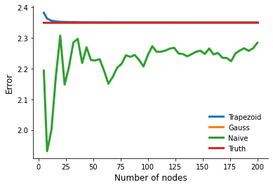
Monte Carlo integration only converges very slowly. Let’s consider our smooth benchmarking example from earlier and compare the naive Monte Carlo approach to the quadrature methods.
[15]:
plot_naive_monte_carlo_error(max_nodes=200)
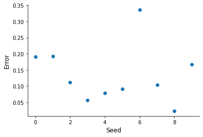
Naive Monte Carlo integration differs from our earlier methods as the approximation itself is a random variable. How about the level of randomness at a given number  of integration nodes?
[16]:
plot_naive_monte_carlo_randomness()
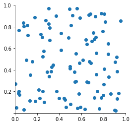
However, Monte Carlo integration is particular useful when tackling multidimensional integrals. Let’s consider the computation of a two dimensional integral going forward.
[17]:
plot_naive_monte_carlo(100)
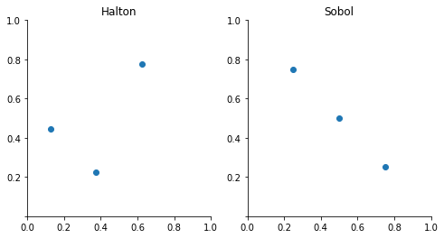
Quasi-Monte Carlo employ deterministic sequences of nodes with the property that
Deterministic sequences of nodes chosen to fill space in a regular manner typically provide more accurate integration approximations than pseudo-random sequences. These sequences are readily available in the chaospy package. The documentation of the package also includes a tutorial on Monte Carlo integration.
[18]:
plot_quasi_monte_carlo(3)
Otherwise, all looks pretty similar to our earlier implementation. Note that the default rule actually takes us back to the naive Monte Carlo method.
[19]:
??monte_carlo_quasi_two_dimensions
Signature: monte_carlo_quasi_two_dimensions(f, a=0, b=1, n=10, rule='random')
Source:
def monte_carlo_quasi_two_dimensions(f, a=0, b=1, n=10, rule="random"):
    """Return Monte Carlo example (two-dimensional).

    Corresponds to naive Monthe Carlo for `rule='random'`. Restricted to same
    integration domain for both variables.
    """
    distribution = cp.J(cp.Uniform(a, b), cp.Uniform(a, b))
    samples = distribution.sample(n, rule=rule).T
    volume = (b - a) ** 2

    fvals = np.tile(np.nan, n)
    weights = np.tile(1 / n, n)

    for i, xval in enumerate(samples):
        fvals[i] = f(xval)

    return volume * np.sum(weights * fvals)
File:      ~/external-storage/sciebo/office/OpenSourceEconomics/teaching/scientific-computing/course/lectures/integration/integration_algorithms.py
Type:      function
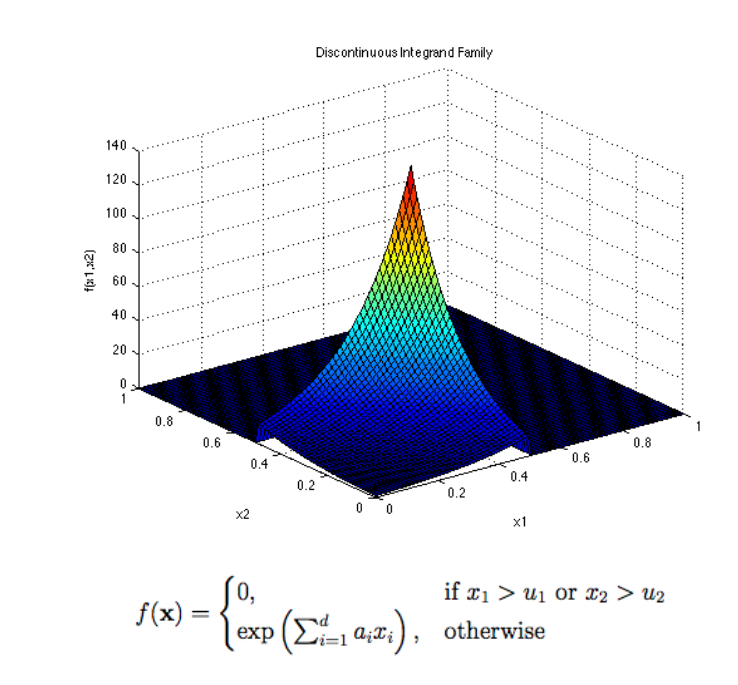
Let’s consider the following test function from Genz (1984).
Exercises
What are the properties of the function?
Compare the performance naive and quasi Monte Carlo integration routines for
 and
and  over the two-dimensional unit cube.
How does Gauss-Legendre quadrature perform?
Applying the integration routines to functions with other input arguments can be achieved with some small modifications. Here we pass in our benchmarking function without any default arguments to a modified naive Monte Carlo integration routine.
[20]:
def genz_discontinuous_no_defaults(x, u, a):
    if x[0] > u[0] or x[1] > u[1]:
        return 0
    else:
        return np.exp((a * x).sum())


def monte_carlo_naive_with_args(f, args=(), a=0, b=1, n=10, seed=128):
    np.random.seed(seed)
    xvals = np.random.uniform(low=a, high=b, size=2 * n).reshape(n, 2)
    volume = (b - a) ** 2

    fvals = np.tile(np.nan, n)
    weights = np.tile(1 / n, n)

    for i, xval in enumerate(xvals):
        # Here is the main modification that passes in the arguments by position now.
        fvals[i] = f(xval, *args)

    return volume * np.sum(weights * fvals)


u, a = (0.5, 0.5), (5, 5)
rslt = monte_carlo_naive_with_args(genz_discontinuous_no_defaults, args=(u, a))
Resources
Research
https://www.sciencedirect.com/science/article/abs/pii/S0304407607002552
Philip J. Davis and Philip Rabinowitz, Methods of Numerical Integration.
https://www.sciencedirect.com/science/article/pii/S0021999185712090
https://ins.uni-bonn.de/media/public/publication-media/sparse_grids_nutshell.pdf?pk=639
Other resources
http://hplgit.github.io/prog4comp/doc/pub/p4c-sphinx-Python/._pylight004.html
http://people.duke.edu/~ccc14/cspy/15C_MonteCarloIntegration.html
https://www.math.ubc.ca/~pwalls/math-python/integration/integrals/
https://guido.vonrudorff.de/wp-content/uploads/2020/05/NumericalIntegration.pdf
https://readthedocs.org/projects/mec-cs101-integrals/downloads/pdf/latest/
References
Genz, A. (1984, September). Testing multidimensional integration routines. In Proc. of international conference on Tools, methods and languages for scientific and engineering computation (pp. 81-94). Elsevier North-Holland, Inc..